IP3 and Intermodulation Distortion: IIP3, OIP3, Formulas, and Measurement

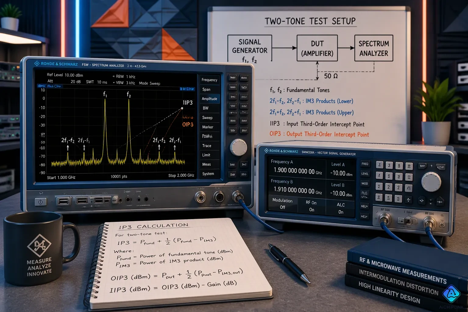
IP3, also called the third order intercept point or TOI, is an estimated figure of merit for weakly nonlinear devices such as amplifiers, mixers, and receivers. This metric goes with a distortion mechanism: two or more tones mix into new products near the original frequencies. Those products corrupt the wanted signal, so engineers track IP3 and intermodulation distortion during design and test. Strong nearby signals can bury a weak one, and the intercept point predicts how soon that happens. This article explains the difference between IIP3 and OIP3, gives the key conversion formulas, and walks through the two-tone measurement procedure step by step.

Key Takeaways

• IP3 is an estimated number that shows how linear a device is. It is not a power level you can measure directly.

• IIP3 and OIP3 describe the same intercept point, one at the input and one at the output; OIP3 = IIP3 + Gain (in dB).

• Third-order intermodulation products show up close to the original signals, so they are hard to filter out.

• A clean two-tone test with low distortion and good isolation gives accurate IP3 measurements.

• A higher OIP3 means better linearity and a stronger ability to resist intermodulation distortion.

IP3 and Intermodulation Distortion Basics

IM3 Products and Frequencies

IP3 and intermodulation distortion explain what happens when two or more signals go through a device that is only weakly nonlinear, like a linear amplifier or a mixer. The device mixes the tones and makes new frequencies. You get the order of each product by adding up the harmonic multiplying constants of the two input frequencies. A product like f1 + f2 is second order, while 2f1 − f2 is third order. The two third-order intermodulation products that matter most show up at these frequencies:

Intermodulation Product	Frequency Formula
Third-order IM product (1)	2f1 − f2
Third-order IM product (2)	2f2 − f1

These third-order intermodulation products land only one tone spacing away from the fundamentals. With input tones at 900 MHz and 901 MHz, the IM3 products show up at 899 MHz and 902 MHz. Each one sits just 1 MHz from its nearest fundamental. Filtering is the usual fix, but it fails here.

The most troublesome intermodulation products are 2f1 ± f2 and 2f2 ± f1 because these frequencies are very close to the fundamental frequency. Filtering becomes hard when the products are very close in frequency to the fundamental signals.

An in-band IM3 product cannot be removed without also weakening wanted channels. Designers control it with higher-linearity parts, lower signal levels, and more compression margin.

IP3 as an Extrapolated Metric

The third order intercept point is not a power level you can measure directly. It is an extrapolated meeting point of intermodulation distortion products in the desired output. Engineers get it by plotting output power against input power on logarithmic scales. The fundamental follows a straight line with slope 1. The third-order product rises 3 dB for every 1 dB of input increase, which gives a slope of 3. Extending both lines to where they cross gives the intercept point, read from the input axis as IIP3 or the output axis as OIP3.

A common mistake is fitting the lines to data taken at too high a power level. The intercept point should come from measured data at the lowest possible power level, limited only by instrument or device noise. This measurement discipline keeps the extrapolation honest.

Third Order Intercept Point: IIP3 vs. OIP3

IIP3 and OIP3 Definitions

The third order intercept point ip3 describes one model, seen from two reference planes. The input-referred third-order intercept point, or IIP3, is the extrapolated intercept read on the input axis. The output-referred third-order intercept point, or OIP3, is the same crossing point read on the output axis. Both values describe the same device behavior. Only the reference plane is different.

The input IP3 (IIP3) is just the OIP3 minus the gain of the amplifier — that is, IIP3 = OIP3 − G, which rearranges to OIP3 = IIP3 + G.

The addition works because all three quantities are logarithmic. Gain in dB simply shifts the input-referred intercept to the output plane. A stage with gain GdB, measured at the same frequency, load, and gain state in the linear region, follows OIP3dBm ≈ IIP3dBm + GdB. Mixing up input-referred and output-referred IP3 is a common error. Always state the reference plane, because mixing them causes gain-magnitude errors.

A spectrum analyzer screen gives a second route to the output intercept point. Here OIP3 = POUT + ΔP/2, where POUT is the fundamental signal power and ΔP = POUT − POUT_3, the gap between the fundamental and the third-order intermodulation product.

IP3 Calculation Examples

A worked example makes the arithmetic concrete. Two tones of -20 dBm each enter an amplifier with 15 dB gain. Each tone exits at -5 dBm, and the IM3 products sit at -65 dBm, giving ΔIM = 60 dB.

Quantity	Value
Input tone power	-20 dBm each
Output tone power (POUT)	-5 dBm each
IM3 product power	-65 dBm
ΔP	60 dB
OIP3	25 dBm
IIP3	10 dBm

The calculation runs in two steps. First, OIP3 = -5 + 30 = 25 dBm. Second, IIP3 = 25 - 15 = 10 dBm, which confirms OIP3 = IIP3 + G (25 = 10 + 15).

Engineers also work backward from a requirement. Suppose a receiver must keep intermodulation products below a set level at a known input power. The designer adds half the required suppression margin to the tone power to find the needed OIP3, then subtracts gain to obtain the required IIP3 for part selection.

OIP3 also signals when the IM3 product becomes significant. In RADAR receivers, weak returns arrive alongside strong nearby echoes. A low output intercept point lets intermodulation products rise above the noise floor at lower signal levels, so the receiver loses small targets sooner.

IP3 Measurement Calculation and Two-Tone Test

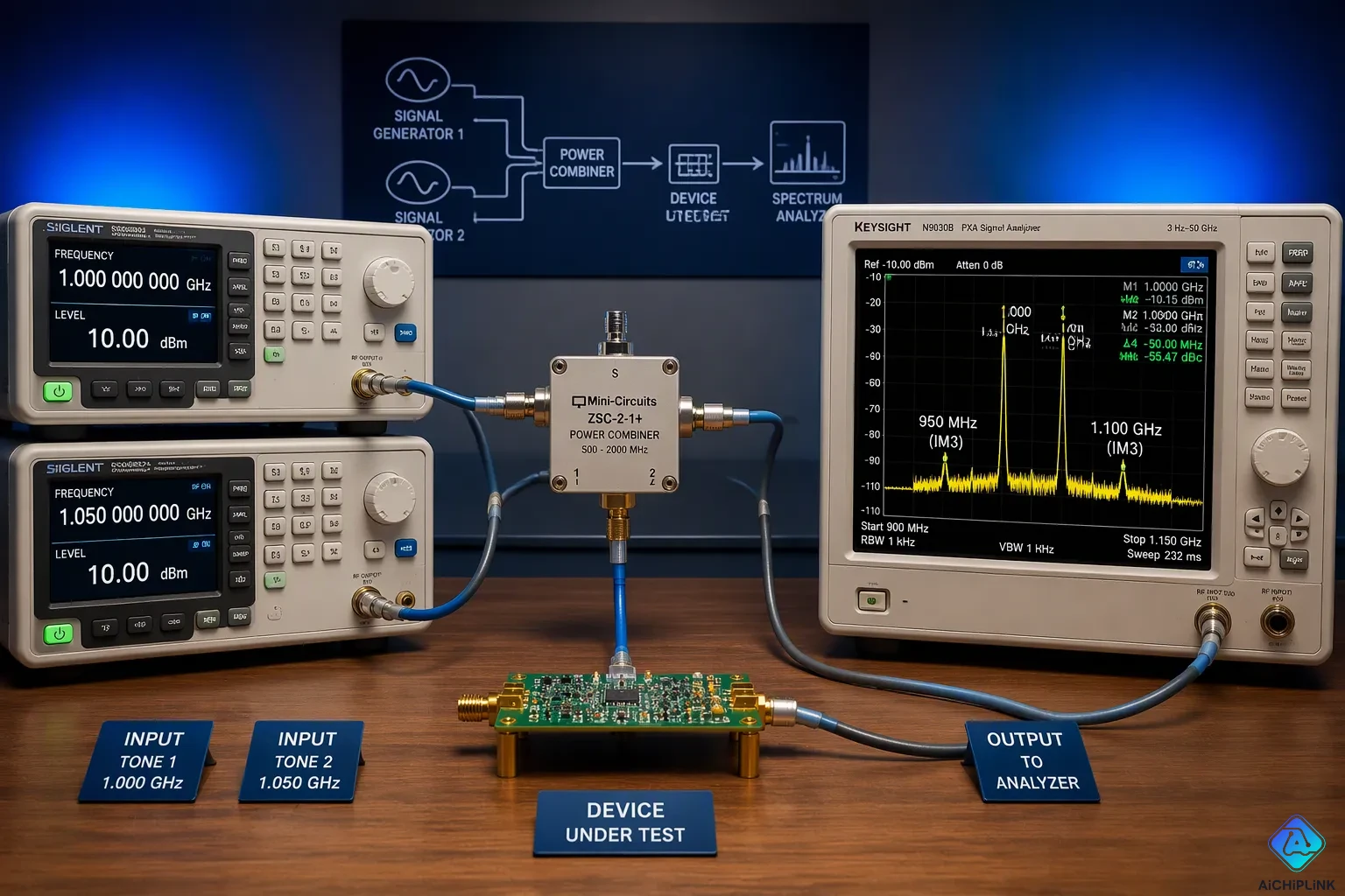
Two-Tone Test Setup

A two-tone test needs two signal generators, a power combiner, the device under test, and a spectrum analyzer. This method sends two equal tones into the input and reads the output spectrum. Tone spacing depends on the analyzer and the goal. An FSIQ analyzer quoting an IMD spec needs spacing above 5 times the resolution bandwidth or 10 kHz, whichever is greater, with tones at -30 dBm. An R&S FSW or FSV avoids ADC intermodulation when spacing exceeds 5 MHz, because both tones then stay out of the ADC input at once. A fixed spacing setup keeps CW tones near full-scale ADC level. A swept analyzer with a wideband digital IF pairs wide spacing with a very narrow span.

The procedure runs in order. Set both generators to equal power and confirm the combiner loss. Drive the DUT well below compression. Capture the fundamental and the third-order intermodulation products on the analyzer. A single measurement point is enough for the ip3 measurement calculation, since OIP3 = P_f + ΔP/2, where P_f is the fundamental power and ΔP is the gap to the IM3 level. One point cannot verify the 3:1 slope of fundamental versus IM3, so sweep power across several points when slope matters.

Measurement Errors and Fixes

Several errors corrupt two-tone ip3 data. Instrument nonlinearity is the first. A VNA receiver may report its own IIP3 instead of the DUT's OIP3, so pad the receiver input to keep levels between -10 and -15 dBm. Insufficient tone isolation is the second. Poor combiner isolation lets one tone leak into the other source and mix, which creates spurious IM tones. Use a resistive combiner such as a Wilkinson power divider with greater than 20 dB isolation between generator ports. Add a directional coupler or isolator on each generator output to block source-to-source coupling.

Compression is the third error. The test extrapolates IP3 from IM levels 40 to 60 dBc below the fundamentals, and hard limiting invalidates that extrapolation. Keep the IM3 tones in the 40 to 60 dBc range. Setup verification is the fourth. Run the setup without the DUT at expected output levels. Residual IM tones should sit 20 to 30 dB below the DUT-generated IM tones. Careful setup matters because artifacts can make the DUT appear better or worse than it is, and ip3 measurement accuracy depends on clean measured intermodulation product levels. These checks protect the calculated ip3 and keep the two-tone test trustworthy.

IP3 vs. P1dB and Component Selection

P1dB and IP3 show two different sides of nonlinearity. P1dB is the output power where gain drops 1 dB from its small-signal value, and it marks where serious nonlinear behavior begins. IP3 is an estimated small-signal number built from two-tone intermodulation products. The table below compares the two.

Attribute	P1dB	IP3
Nature of measure	Measured large-signal, single-tone gain-compression point	Extrapolated small-signal, two-tone intermodulation figure
Signal regime	Device already significantly nonlinear at the measurement point	Derived from low-level IM3 products growing at a predictable 3:1 slope
Physical reachability	Directly measured on the compression curve	Normally never reached physically; hypothetical intersection of extrapolated fundamental and IM3 outputs

P1dB matters more when one strong tone or blocker drives the device, and when compression effects like spectral regrowth and EVM degradation take over. IP3 matters more for weak-signal cases where intermodulation products near the wanted channel set the limit.

Cascaded IP3 and Gain

A cascade does not average stage linearity. Gain distribution controls the result. Each stage boosts the signal and pushes later stages closer to nonlinear operation. The final stage usually controls overall IP3 because signal levels are highest there. For an n-stage chain, the system OIP3 follows a reciprocal sum: 1/OIP3_sys = 1/OIP3_n + 1/(OIP3_(n−1)·G_n) + …, where each OIP3 is in mW and each G is linear power gain, not dB. Convert dBm to mW before computing, then convert back.

Putting high gain early lowers noise figure but hurts cascaded IP3. Designers add attenuators between stages, pick high-OIP3 mixers and amplifiers, or cut early gain to avoid overdriving later parts.

Comparing IP3 Specifications

Datasheet IP3 values are virtual parameters, estimated from other specs, so the basis for that estimate matters during comparison. Check the reference plane, tone spacing, and power level behind each number. A useful cross-check: OIP3 usually sits 9–15 dB above P1dB for bipolar and FET amplifiers. A datasheet claim far outside that range deserves a closer look. Higher OIP3 means better linearity and stronger resistance to intermodulation distortion, so compare parts at the same gain state and frequency.

Engineers should think of IP3 as an estimated number, not a power level they can measure directly. The model depends on the 3:1 slope between the fundamental and IM3 output, so the intercept point stays hypothetical.

The formula OIP3 = IIP3 + G connects the input and output reference planes. The IM3 products at 2f1 − f2 and 2f2 − f1 land one tone spacing away from the fundamentals, and filtering cannot remove them without harming wanted channels. This fact drives the study of ip3 and intermodulation distortion.

Trustworthy data requires a clean two-tone setup and awareness of common measurement errors. Instrument nonlinearity, poor tone isolation, and compression all corrupt intermodulation products. Careful checks keep the reported ip3 honest.

 

 

 

 

 

Written by Jack Elliott from AIChipLink.

 

AIChipLink, one of the fastest-growing global independent electronic   components distributors in the world, offers millions of products from thousands of manufacturers, and many of our in-stock parts is available to ship same day.

 

We mainly source and distribute integrated circuit (IC) products of brands such as Broadcom, Microchip, Texas Instruments, Infineon, NXP, Analog Devices, Qualcomm, Intel, etc., which are widely used in communication & network, telecom, industrial control, new energy and automotive electronics. 

 

Empowered by AI, Linked to the Future. Get started on AIChipLink and submit your RFQ online today!