What You Need to Know About Nanofarad and Capacitance

Introduction

Pick up any PCB schematic and you will see them everywhere — 100nF, 10nF, 47nF. Capacitors measured in nanofarads are among the most common passive components in all of electronics, appearing in virtually every digital, analog, RF, and power circuit ever designed. Yet for many students, hobbyists, and even experienced engineers crossing into a new design domain, the nanofarad (nF) remains a source of persistent confusion: Is 100nF the same as 0.1µF? What does the code "104" stamped on a ceramic disc mean? When should you use a 10nF instead of a 100pF? How does capacitance affect filter frequency?

This guide answers all of those questions. From first principles — what capacitance actually is and why the farad is defined the way it is — through the complete nF-to-pF-to-µF conversion system, practical circuit applications, capacitor marking codes, measurement techniques, and selection criteria, this is the most complete reference on nanofarads and capacitance you will find in one place.

According to IEC 60027-2 (Letter Symbols for Physical Quantities), the internationally standardized system for electrical units, the nanofarad (nF) is the preferred expression for capacitance values between 1,000 pF and 1,000,000 pF — the range used by the majority of signal-conditioning, timing, filtering, and decoupling capacitors in modern electronic circuits. Mastering this unit and its relationships is not optional for anyone working seriously with electronics.

---

1.0 What Is Capacitance? The Fundamentals

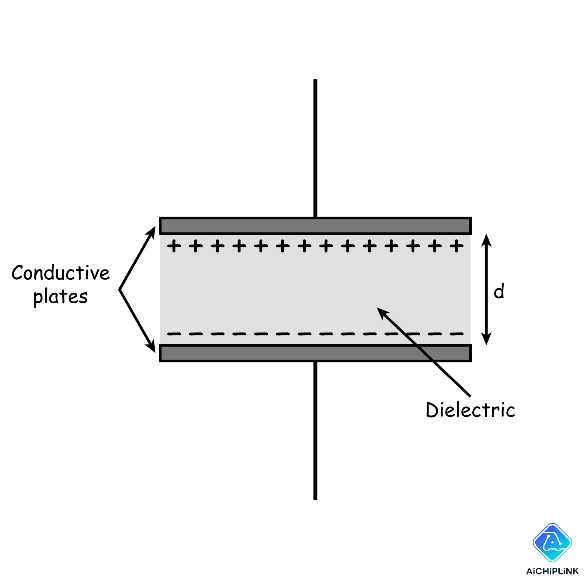
Capacitance is the ability of a component or system to store electric charge in response to an applied voltage. The fundamental physics is straightforward: when a voltage (V) is applied across a capacitor, electric charge (Q) accumulates on its conductors. The ratio of charge stored to voltage applied is the capacitance (C):

C = Q / V

where C is in farads, Q is in coulombs, and V is in volts.

A capacitor with higher capacitance stores more charge per volt of applied voltage — it can absorb a larger quantity of energy and release it later. This energy storage and release mechanism is the foundation of every capacitor application: smoothing voltage ripple, coupling AC signals while blocking DC, setting timing constants in RC circuits, and storing energy in switched-mode power supplies.

---

1.1 The Farad: SI Unit of Capacitance

The farad (F) is the SI (International System) base unit of electrical capacitance, named after the English scientist Michael Faraday (1791–1867), who conducted foundational experiments on electromagnetism and electrochemistry in the 19th century. The formal definition:

One farad is the capacitance of a capacitor that stores one coulomb of charge when one volt is applied across it.

One farad is, practically speaking, an enormous quantity of capacitance. A 1 F capacitor built from conventional dielectric materials would be physically enormous — too large for any practical PCB-mounted application. Modern supercapacitors (also called ultracapacitors or electric double-layer capacitors) achieve tens to thousands of farads in physically compact cells, but these are specialized energy storage devices, not general-purpose signal capacitors. The capacitors used in everyday electronic circuits range from millionths to billionths of a farad — which is exactly why the sub-unit prefixes (micro-, nano-, pico-) exist.

---

1.2 The Capacitance Unit Hierarchy: pF, nF, µF, mF, F

The complete standard prefix hierarchy for capacitance, from smallest to largest:

Unit	Symbol	Power of 10	Fraction of a Farad	Typical Capacitor Types
Picofarad	pF	10⁻¹²	0.000 000 000 001 F	RF/microwave ceramics, trimmer caps, crystal load caps
Nanofarad	nF	10⁻⁹	0.000 000 001 F	MLCC, film caps (timing, filtering, coupling, decoupling)
Microfarad	µF	10⁻⁶	0.000 001 F	Electrolytic, tantalum, large MLCC (power supply, bulk decoupling)
Millifarad	mF	10⁻³	0.001 F	Large electrolytics, some film caps (rarely used as unit)
Farad	F	10⁰	1 F	Supercapacitors/ultracapacitors (energy storage)

The three units you will use in virtually every electronic circuit are pF, nF, and µF. Each successive unit is exactly 1,000 times larger than the previous — the base-1000 (10³) relationship that makes conversions systematic and predictable.

---

1.3 What Exactly Is a Nanofarad (nF)?

The nanofarad (nF) is one-billionth (10⁻⁹) of a farad. The prefix "nano" comes from the Greek word "nanos" (νᾶνος, meaning dwarf), standardized as the SI prefix for 10⁻⁹ by the 11th General Conference on Weights and Measures in 1960.

1 nF = 10⁻⁹ F = 0.000 000 001 F

In practical terms, the nanofarad is the "middle" of the three common capacitance units — larger than picofarads (used for very high-frequency RF applications) and smaller than microfarads (used for power supply bulk storage). This middle position makes nanofarad-range capacitors the most versatile in electronics: fast enough to respond to frequencies up to tens of megahertz, yet large enough to store sufficient charge for timing, coupling, and noise-filtering functions that picofarad values cannot perform.

A useful physical intuition: a 1 nF capacitor charged to 5 V stores 5 nanocoulombs (nC) of charge — enough to briefly power a modern low-power microcontroller for approximately 0.001 µs. Not much in absolute terms, but in a bypass capacitor application, those nanocoulombs are delivered to the IC's power pin in nanoseconds during a logic transition, before the longer-path supply inductance can respond. That speed-of-delivery function is what makes nF capacitors indispensable.

The nanofarad is used slightly differently across different engineering traditions. In North America and the UK, "nF" is the standard notation. In some European and older Japanese/German engineering documents, the same values may be expressed as fractions of a microfarad (0.001 µF for 1 nF) or as large picofarad values (1000 pF for 1 nF) — which is why conversion fluency matters even when working from well-known designs.

---

1.4 Capacitive Reactance: How Capacitance Affects AC Circuits

A capacitor's behavior in AC circuits is characterized by its capacitive reactance (XC) — the opposition to alternating current flow. Unlike a resistor (whose opposition is constant at any frequency), a capacitor's reactance decreases as frequency increases:

XC = 1 / (2π × f × C)

where XC is in ohms, f is in hertz, and C is in farads.

Practical implications for nF capacitors:

Capacitor	XC at 1 kHz	XC at 100 kHz	XC at 10 MHz
1 nF	159 kΩ	1.59 kΩ	15.9 Ω
10 nF	15.9 kΩ	159 Ω	1.59 Ω
100 nF	1.59 kΩ	15.9 Ω	0.159 Ω
470 nF	338 Ω	3.38 Ω	0.034 Ω

This table reveals immediately why nanofarad capacitors are ideal for mid-frequency applications. A 100 nF capacitor has a reactance of about 1.6 kΩ at 1 kHz (high impedance — blocks low-frequency noise effectively) but only 16 Ω at 100 kHz (low impedance — passes or bypasses high-frequency signals easily). This is the mathematical basis for their use as decoupling capacitors: they present low impedance to switching transients (100 kHz–100 MHz) while offering high impedance to DC and low-frequency signals.

---

2.0 Nanofarad Conversion: Complete Reference Tables

2.1 Core Conversion Formulas: nF ↔ pF ↔ µF ↔ F

All conversions between pF, nF, µF, and F follow the base-1000 step relationship. Memorize these four rules and you will never need a conversion chart again:

nF to pF: Multiply by 1,000 X nF × 1,000 = X,000 pF Example: 4.7 nF × 1,000 = 4,700 pF

nF to µF: Divide by 1,000 X nF ÷ 1,000 = 0.00X µF Example: 100 nF ÷ 1,000 = 0.1 µF

nF to F: Divide by 1,000,000,000 (= × 10⁻⁹) X nF ÷ 10⁹ = X × 10⁻⁹ F Example: 10 nF = 10 × 10⁻⁹ F = 0.00000001 F

µF to nF: Multiply by 1,000 X µF × 1,000 = X,000 nF Example: 0.47 µF × 1,000 = 470 nF

pF to nF: Divide by 1,000 X pF ÷ 1,000 = 0.00X nF Example: 2,200 pF ÷ 1,000 = 2.2 nF

pF to µF: Divide by 1,000,000 X pF ÷ 1,000,000 = X × 10⁻⁶ µF Example: 100,000 pF ÷ 1,000,000 = 0.1 µF

---

2.2 Master Conversion Table: Common Capacitor Values

The following table covers all standard capacitor values you will encounter in real-world designs, expressed simultaneously in pF, nF, and µF for instant cross-reference:

pF	nF	µF	Notes
1 pF	0.001 nF	0.000001 µF	RF/load capacitors, crystal matching
10 pF	0.01 nF	0.00001 µF	RF tuning, VCO, crystal load
22 pF	0.022 nF	0.000022 µF	Crystal load capacitor (common 18–22 pF)
47 pF	0.047 nF	0.000047 µF	RF filter, impedance matching
100 pF	0.1 nF	0.0001 µF	Bypass, RF decoupling
220 pF	0.22 nF	0.00022 µF	Snubber, EMI filter
470 pF	0.47 nF	0.00047 µF	RC timing, HF filter
1,000 pF	1 nF	0.001 µF	Boundary pF/nF; signal coupling
2,200 pF	2.2 nF	0.0022 µF	Filter, debounce
4,700 pF	4.7 nF	0.0047 µF	Snubber, EMI
10,000 pF	10 nF	0.01 µF	Decoupling, RC timer
22,000 pF	22 nF	0.022 µF	Audio coupling
47,000 pF	47 nF	0.047 µF	Switch debounce, filter
100,000 pF	100 nF	0.1 µF	Universal decoupling — most common capacitor in electronics
220,000 pF	220 nF	0.22 µF	Power rail decoupling
470,000 pF	470 nF	0.47 µF	Low-frequency filter
1,000,000 pF	1,000 nF	1 µF	Boundary nF/µF; bulk bypass
—	—	4.7 µF	Bulk bypass, LDO output
—	—	10 µF	Power supply filter
—	—	100 µF	Large bypass, reservoir cap
—	—	1,000 µF	Power supply reservoir

Key equivalences to memorize:

• 100 nF = 0.1 µF = 100,000 pF — the most commonly used decoupling capacitor value in all of electronics
• 1 nF = 1,000 pF — the boundary value between the pF and nF ranges
• 1,000 nF = 1 µF — the boundary value between the nF and µF ranges

---

2.3 Worked Conversion Examples

These examples cover the most common real-world scenarios where nF conversion is needed:

Example 1: Reading a schematic that mixes units A schematic shows a coupling capacitor as "0.01 µF" but your distributor lists values in nF. Convert: 0.01 µF × 1,000 = 10 nF — order a 10 nF capacitor.

Example 2: Decoding a datasheet timing specification A timer IC datasheet says: "For a 1 ms time constant, use RT = 10 kΩ and CT = 0.1 µF." You want to verify in nF: 0.1 µF × 1,000 = 100 nF — use a 100 nF capacitor.

Example 3: Cross-referencing component datasheets One capacitor is marked "4700 pF" on its body. A circuit diagram calls for "4.7 nF." Are they the same? 4700 pF ÷ 1,000 = 4.7 nF — yes, identical.

Example 4: Calculating capacitive reactance for a 100 nF decoupling capacitor at 10 MHz XC = 1 / (2π × 10 × 10⁶ × 100 × 10⁻⁹) = 1 / (2π × 1) = 0.159 Ω At 10 MHz, a 100 nF capacitor presents only 0.159 Ω of reactance — nearly a short circuit for high-frequency noise.

Example 5: European-style notation An older German schematic shows "n47" — what does this mean? In European notation, the letter "n" indicates nanofarads and its position marks the decimal point: "n47" = 0.47 nF, "4n7" = 4.7 nF, "47n" = 47 nF.

---

3.0 Where Nanofarad Capacitors Are Used

3.1 Filtering and Decoupling Applications

The most common use of nF capacitors is as decoupling and bypass capacitors on integrated circuit power supply pins. Every time an IC switches its logic outputs, it draws a brief spike of current from its power supply. If that current spike must travel even a few centimeters of PCB trace to reach the power supply output, the trace inductance creates a momentary voltage dip on the IC's VCC pin — exactly when the IC needs clean, stable power.

A 100 nF ceramic capacitor placed within 1–2 mm of the IC's VCC pin acts as a local charge reservoir — it supplies the transient current demand instantly, before the inductance of the longer power trace can respond. The 100 nF value is chosen because its capacitive reactance at 10–100 MHz (the typical IC switching frequency range) is 0.2–2 Ω — low enough to provide a near-short-circuit path to ground for switching current transients.

Beyond IC decoupling, nF capacitors appear in RC low-pass filters to block high-frequency switching noise from power supplies from reaching sensitive analog circuits. A 10 nF capacitor in parallel with the supply pin of a precision ADC provides additional noise suppression at 100 kHz–100 MHz beyond what the bulk 10 µF capacitor contributes.

---

3.2 Timing Circuits and RC Networks

The RC time constant — the product of a resistor and capacitor — determines the charging and discharging time of capacitor circuits. For a nF-range capacitor with a kilohm-range resistor, the resulting time constants fall in the microsecond-to-millisecond range, ideal for:

• Switch debouncing: A 10 nF capacitor with a 10 kΩ resistor creates a 100 µs time constant — long enough to filter mechanical contact bounce (1–50 µs) while short enough to respond to a deliberate keypress within 1 ms
• Monostable timers: 555 timer circuits use nF capacitors to set pulse widths in the microsecond range for tone generation, pulse-width control, and event timing
• Phase-locked loop (PLL) loop filters: nF capacitors in the loop filter set the bandwidth of the phase detector's output, determining PLL lock speed
• Sample-and-hold circuits: A nF-range sampling capacitor stores the analog voltage sample during the hold phase

The time constant formula: τ = R × C

For R = 100 kΩ, C = 100 nF: τ = 100,000 × 0.0000001 = 10 ms — a 10 millisecond time constant, suitable for human-interface timing such as button debouncing and LED pulse shaping.

---

3.3 RF and High-Frequency Signal Coupling

In RF and audio circuits, nF capacitors serve as AC coupling (DC-blocking) elements — they pass the AC signal while blocking any DC bias voltage that would shift the operating point of downstream stages.

In an audio amplifier, a 100 nF coupling capacitor with a 1 kΩ load creates a high-pass filter with a −3 dB cutoff frequency of:

f_cutoff = 1 / (2π × R × C) = 1 / (2π × 1000 × 0.0000001) = 1,592 Hz

This 1.6 kHz cutoff is appropriate for speech-band audio. Increasing the coupling capacitor to 1,000 nF (1 µF) lowers the cutoff to 159 Hz, extending bass reproduction.

For RF signal coupling at 100 MHz, a 10 nF capacitor has a reactance of only 0.16 Ω — effectively a short circuit at RF frequencies, passing the signal with negligible insertion loss while still blocking DC bias.

📺 Recommended Watch: Understanding Capacitance: nF, pF, µF Explained Visually

<iframe width="560" height="315" src="https://www.youtube.com/embed/placeholder_capacitance_nF_explained" title="Capacitance Units Explained: Nanofarad Picofarad Microfarad - Conversions and Applications" frameborder="0" allow="accelerometer; autoplay; clipboard-write; encrypted-media; gyroscope; picture-in-picture; web-share" referrerpolicy="strict-origin-when-cross-origin" allowfullscreen></iframe>

This video visually explains the farad, nanofarad, picofarad, and microfarad units; demonstrates unit conversion with worked examples; and shows real circuit applications for each capacitance range.

---

3.4 Capacitor Types Used in the nF Range

The nanofarad range is served primarily by two capacitor technology families:

Multi-Layer Ceramic Capacitors (MLCC): The dominant technology for nF-range capacitors in modern electronics. MLCCs consist of alternating layers of ceramic dielectric and metal electrodes, stacked and fired to form a monolithic chip. Key characteristics: small size (0201, 0402, 0603 packages), very low ESR and ESL for excellent high-frequency performance, no polarity, and a wide range of dielectric types.

Dielectric types matter significantly for nF MLCC selection: C0G/NP0 is ultra-stable (±30 ppm/°C) and low-loss — ideal for precision timing and RF applications but limited to values below ~10 nF in small packages. X7R offers ±15% capacitance variation over −55°C to +125°C and is the standard choice for decoupling and general filtering in the 10 nF to 1 µF range. X5R is similar to X7R but rated to +85°C only. Y5V and Z5U offer high capacitance density but exhibit ±20–80% variation with temperature and DC bias — avoid these for any application where capacitance stability matters.

Film Capacitors (Polyester, Polypropylene, PPS): Used in the nF range where tighter tolerance, lower loss, or higher voltage rating than MLCC is needed. Common in audio circuits (polyester film coupling capacitors), EMI suppression (X/Y-class safety-rated film capacitors rated for line voltage), and precision timing where the capacitor's value must remain stable over millions of cycles.

In the nF range, avoid electrolytic capacitors — they are polarized, physically large relative to their capacitance, have high ESR, and are optimized for the µF–mF range where their high capacitance density is needed.

---

4.0 Reading Capacitor Codes, Measuring & Selecting

4.1 Decoding 3-Digit Capacitor Marking Codes

Small ceramic capacitors are typically marked with a 3-digit numerical code rather than the full value. The decoding rule:

• First two digits = significant figures of the value in picofarads
• Third digit = number of zeros to add (power-of-10 multiplier)

Decoded value = (first two digits) × 10^(third digit) picofarads

Common codes decoded:

Code	Decoded (pF)	Equivalent nF	Equivalent µF
100	10 × 10⁰ = 10 pF	0.01 nF	0.00001 µF
101	10 × 10¹ = 100 pF	0.1 nF	0.0001 µF
102	10 × 10² = 1,000 pF	1 nF	0.001 µF
103	10 × 10³ = 10,000 pF	10 nF	0.01 µF
104	10 × 10⁴ = 100,000 pF	100 nF	0.1 µF
222	22 × 10² = 2,200 pF	2.2 nF	0.0022 µF
223	22 × 10³ = 22,000 pF	22 nF	0.022 µF
472	47 × 10² = 4,700 pF	4.7 nF	0.0047 µF
473	47 × 10³ = 47,000 pF	47 nF	0.047 µF
474	47 × 10⁴ = 470,000 pF	470 nF	0.47 µF

The single most important code to memorize: "104" = 100 nF = 0.1 µF — the ubiquitous decoupling capacitor code found on countless PCBs worldwide.

Tolerance suffix codes often appear after the 3-digit number: J = ±5%, K = ±10%, M = ±20%. Example: "104K" = 100 nF ±10%.

---

4.2 Standard E-Series Values in the nF Range

Capacitors are manufactured in preferred value series (E-series) — logarithmically spaced sets of values defined by IEC 60063. The most commonly stocked nF values you will find at distributors follow the E6 and E12 series:

E6 series (20% tolerance): 1.0, 1.5, 2.2, 3.3, 4.7, 6.8 — repeated at each decade (1 nF, 1.5 nF, 2.2 nF, 3.3 nF, 4.7 nF, 6.8 nF, 10 nF, 15 nF…)

E12 series (10% tolerance): adds 1.2, 1.8, 2.7, 3.9, 5.6, 8.2 between the E6 values.

The most commonly stocked nF values in the industry are: 1 nF, 2.2 nF, 4.7 nF, 10 nF, 22 nF, 33 nF, 47 nF, 100 nF, 220 nF, 470 nF, 1,000 nF (= 1 µF).

If your calculation yields a non-standard value (e.g., 37 nF), round to the nearest E-series value (33 nF or 47 nF) and adjust the companion resistor to maintain the intended time constant or cutoff frequency.

---

4.3 How to Measure Capacitance

Measuring a capacitor's actual capacitance requires either a digital multimeter (DMM) with CAP function or a dedicated LCR meter:

Digital multimeter with CAP function: Connect the capacitor to the CAP test terminals (observe polarity for electrolytic types), select the capacitance range, and read the value. Most modern auto-ranging DMMs measure accurately from 1 nF to 200 µF. Limitation: DMMs measure at 100 Hz or 1 kHz only — they do not capture frequency-dependent behavior or ESR.

LCR meter: The gold standard for capacitor characterization. A bench LCR meter measures capacitance, ESR, dissipation factor (tan δ), and impedance magnitude across selectable test frequencies (100 Hz, 1 kHz, 10 kHz, 100 kHz). Essential for verifying MLCC frequency response, DC bias derating, and dielectric behavior. For production incoming inspection of critical capacitors, an LCR meter is mandatory.

Self-resonant frequency (SRF): Every real capacitor has an SRF above which it becomes inductive rather than capacitive. A 100 nF 0402 MLCC typically has an SRF around 50–100 MHz. Below the SRF the component behaves as a capacitor; above it behaves as an inductor. Always verify the SRF of your chosen capacitor type at the frequencies of interest — Murata, TDK, and other manufacturers publish impedance-vs-frequency curves in their online SimSurfing and online tools.

---

4.4 Key Selection Parameters Beyond Capacitance Value

When specifying an nF capacitor for a production design, the nominal capacitance is only the starting point. These additional parameters are equally important:

Voltage rating (VR): Select a voltage rating at least 1.5–2× the maximum circuit voltage. For a 3.3 V rail, use 6.3 V or 10 V rated capacitors. Be aware that X5R and X7R MLCCs exhibit significant DC bias derating — a 10 V 0402 X7R capacitor at 5 V DC may have only 40–60% of its nominal capacitance due to the electric field reducing the ceramic permittivity. Always verify effective capacitance at operating voltage using the manufacturer's DC bias derating curves.

Dielectric type: C0G/NP0 for stability-critical timing and RF; X7R for general-purpose decoupling and filtering; X5R for commercial temperature range bulk bypass; avoid Y5V/Z5U for any critical application.

ESR (Equivalent Series Resistance): Lower ESR gives better high-frequency performance and lower self-heating under ripple current. Critical for power supply decoupling applications where the capacitor must handle repeated high-frequency current pulses.

Physical package size: Smaller packages (0402, 0201) have lower parasitic inductance (ESL) and higher self-resonant frequencies — use them for decoupling capacitors in high-frequency applications. Larger packages (0805, 1206) support higher maximum capacitance and voltage ratings.

Operating temperature grade: Commercial (0°C to +70°C), industrial (−40°C to +85°C), or automotive AEC-Q200 (−40°C to +125°C or +150°C). Specify the grade that covers the application's full temperature range.

---

5.0 Where to Buy nF Capacitors

Nanofarad-range capacitors are among the most widely available and cost-competitive passive components in the electronics industry. Key sourcing channels and manufacturers:

Authorized distributors: DigiKey, Mouser Electronics, Arrow Electronics, and Avnet offer the widest selection with full parametric search — filter by exact capacitance, voltage rating, dielectric type, package size, and temperature grade. LCSC Electronics offers competitive pricing for prototype and lower-volume production orders.

Leading MLCC manufacturers for nF capacitors:

• Murata GRM series — industry benchmark; GRM155 (0402) and GRM188 (0603) cover 1 nF to 1 µF
• TDK CGA/C series — automotive AEC-Q200 qualified options; CGA series for −55°C to +125°C
• Samsung CL series — high-volume competitive pricing; CL05 (0402) and CL10 (0603) families
• Yageo CC series — cost-effective commercial grade with worldwide availability
• Kemet C series — broad portfolio including specialty dielectrics and high-voltage options

For all your capacitor sourcing needs — from 0402 100 nF X7R decoupling capacitors to precision C0G RF capacitors and automotive-grade AEC-Q200 MLCCs — explore verified inventory with competitive pricing at aichiplink.com.

6.0 Conclusion

The nanofarad is not a complicated unit — it is simply one step in a clean, base-1000 hierarchy running from picofarad through nanofarad to microfarad to farad, each unit exactly 1,000 times larger than the previous. The conversion formulas are straightforward arithmetic once the base relationships are memorized. What gives the nanofarad its outsized importance in electronics is the physical capacitance range it represents — the 1 nF to 1,000 nF window that encompasses the most versatile and widely deployed capacitors in the industry: IC decoupling capacitors, RC timing networks, AC signal coupling elements, noise filter capacitors, and RF bypass components.

Understanding nanofarads deeply means understanding why a 100 nF ceramic capacitor belongs at every IC power pin, how to convert fluently between pF, nF, µF, and F without looking up a chart, what the 3-digit marking code "104" means at a glance, how to select the right dielectric type, voltage rating, and package size for the application at hand, and how capacitive reactance links the nF value to actual circuit behavior across frequencies.

With these skills, the nanofarad transforms from a source of confusion into one of the most intuitive and useful concepts in practical electronics design — and selecting the right nF capacitor for any application becomes a fast, confident engineering decision rather than a guessing game.

For all your capacitor sourcing needs — from 0402 100 nF X7R decoupling capacitors to precision C0G RF capacitors and automotive-grade MLCCs — explore verified inventory with competitive pricing at aichiplink.com.

 

 

 

 

 

Written by Jack Elliott from AIChipLink.

 

AIChipLink, one of the fastest-growing global independent electronic   components distributors in the world, offers millions of products from thousands of manufacturers, and many of our in-stock parts is available to ship same day.

 

We mainly source and distribute integrated circuit (IC) products of brands such as Broadcom, Microchip, Texas Instruments, Infineon, NXP, Analog Devices, Qualcomm, Intel, etc., which are widely used in communication & network, telecom, industrial control, new energy and automotive electronics. 

 

Empowered by AI, Linked to the Future. Get started on AIChipLink.com and submit your RFQ online today!